1 Fundamentals
There are three common patterns of crossed winding, as documented in the literature on basket winding (Wikipedia contributors, n.d.) and early radio coils (Radiomuseum.org, n.d.). They are:
| English | German | Geometry |
|---|---|---|
| basket(-weave) coil | Korbspule | wire alternates inside/outside of \(N\) pegs on a cylinder |
| spider-web coil | Korbbodenspule, Spinnennetzspule, Flachspule | planar version: wire alternates over/under \(N\) radial spokes |
| honeycomb / universal / duo-lateral coil | Honigwabenspule, Wabenspule, Kreuzwickelspule | wire traverses axially while the form rotates, so layers cross in a zig-zag; “honeycomb” = open cross winding with air cells |
All three share one principle: adjacent turns cross at a large angle \(\theta \to 90^\circ\) instead of lying parallel (\(\theta = 0\)):
\[ \theta \uparrow \;\Longrightarrow\; C_d \downarrow,\quad F_\text{prox} \downarrow,\quad f_{sr} \uparrow,\quad Q \uparrow \tag{1.1}\]
They are typically used from about \(50\ \text{kHz}\) up to HF, often wound with Litz wire (HF-Litze). Cotton- or silk-covered wire holds the crossing angles better than enamelled wire, because it has more friction.
1.1 The construction
The different basket winding patterns are closely related to algebra (especially group theory), to geometry (especially Lie groups) and, to some extent, to knot theory (see torus knots).
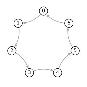
We start by considering the cyclic group \[ C_n = \langle g \mid g^n = e \rangle \;\cong\; \mathbb Z/n\mathbb Z,\qquad g \mapsto 1 . \tag{1.2}\] We can visualise it by its Cayley graph with respect to the generator \(1\). The elements \(0, 1, \dots, n-1\) sit equidistantly on a circle, and an arrow \(j \to j+1\) connects each element to its successor (Figure 1.1).
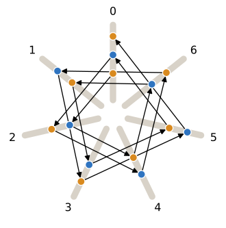
Now fix \(k \in C_n\) and consider the map \[ (-\cdot k) : C_n \to C_n,\qquad j \mapsto j\,k . \tag{1.3}\] Apply it to the successive elements \(0, 1, 2, \dots\); equivalently, add \(k\) again and again. The resulting sequence \(0, k, 2k, 3k, \dots \pmod n\) is the order in which a wire visits the spokes of a spoke form: the spokes are the elements of \(C_n\), and the wire runs from spoke \(jk\) to spoke \((j+1)k\). Figure 1.2 shows this for \((-\cdot 2)\) in \(C_7\), where the wire visits spokes \(0, 2, 4, 6, 1, 3, 5, 0, \dots\) and traces the star polygon \(\{7/2\}\). The map \((-\cdot k)\) of Equation 1.3 is an automorphism of \(C_n\) exactly when \(\gcd(k, n) = 1\); only then does the wire reach every spoke (Corollary 1.1).
CautionCaution: not yet fact-checked
The text has only been fact-checked up to this point. Treat everything that follows as unsubstantiated for now, and proceed with great caution!
1.1.1 Spoke form (spider-web / basket)
Spokes sit at \(\varphi_j = 2\pi j/N\). Index each place the wire passes a spoke by \(k \in \mathbb Z\):
\[ j = k \bmod N \ \text{(spoke)},\qquad n = \lfloor k/N \rfloor \ \text{(turn)},\qquad s = k \bmod 2 \ \text{(side: 0 front, 1 back)} \]
\[ \pi : \mathbb Z \to \mathbb Z_N \times \mathbb Z_2,\qquad k \mapsto (k \bmod N,\ k \bmod 2) \tag{1.4}\]
Theorem 1.1 (Weave condition) The map \(\pi\) in Equation 1.4 is surjective if and only if \(N\) is odd. In that case \[ \mathbb Z_N \times \mathbb Z_2 \cong \mathbb Z_{2N},\qquad \ker\pi = 2N\mathbb Z,\qquad s(n+1, j) = s(n, j) + 1 \pmod 2 . \] Every spoke is passed once in front and once behind, and the pattern has period two turns.
Proof. By the Chinese remainder theorem, \(\mathbb Z_N \times \mathbb Z_2 \cong \mathbb Z_{2N} \iff \gcd(N,2)=1\). The image of \(\pi\) is the cyclic subgroup generated by \((1,1)\), which has order \(\operatorname{lcm}(N,2)\). This equals \(2N\) exactly when \(N\) is odd. For \(N\) even, \(\operatorname{im}\pi \cong \mathbb Z_N\) has index 2 and \(s\) depends on \(j\) alone. All turns then lie on the same side of each spoke and stack in parallel, so there is no weave.
1.1.2 Skip winding (step of \(m\) spokes)
\[ \pi_m : k \mapsto (mk \bmod N,\ k \bmod 2),\qquad \operatorname{ord}\big((m,1)\big) = \operatorname{lcm}\!\Big(\tfrac{N}{\gcd(m,N)},\, 2\Big) \tag{1.5}\]
Corollary 1.1 All spokes are visited \(\iff \gcd(m,N) = 1\). There is a full weave (\(\operatorname{ord} = 2N\)) \(\iff \gcd(m,N) = 1 \wedge N\) odd. The parity of \(m\) does not matter: for example \(N=9\), \(m=2\) works. The number of admissible steps is \(\varphi(N)\) (Euler’s totient), or \(\varphi(N)/2\) up to winding direction (\(m \sim N-m\)). For example, \(\varphi(9)=6\), \(\varphi(11)=10\), \(\varphi(13)=12\).
1.1.3 Symmetry group
Let \(r\) be the rotation by \(2\pi/N\) and \(\sigma_h\) the reflection in the plane of the form. Since \([r,\sigma_h]=1\), \[ \langle r, \sigma_h \rangle = C_{Nh} \cong \mathbb Z_N \times \mathbb Z_2 . \]
Proposition 1.1 For \(N\) odd, \(C_{Nh}\) is cyclic, generated by the rotoreflection \(S_N = r\sigma_h\): \[ \operatorname{ord}(S_N) = 2N,\qquad S_N^{\,2} = r^2,\qquad S_N^{\,N} = \sigma_h,\qquad \langle S_N\rangle = C_{Nh}\cong \mathbb Z_{2N}. \]
Acting on spoke passes, \(S_N : k \mapsto k+1\), so the woven pattern is one orbit of \(\langle S_N\rangle\). Ignoring the radial growth of the spiral, \(\sigma_h = S_N^{\,N} : k \mapsto k+N\) maps turn \(n\) to turn \(n+1\).
1.1.4 Crossing angle (cylindrical basket coil)
Let \(R\) be the radius of the peg circle, \(d_p\) the peg diameter and \(d\) the wire diameter. Between adjacent pegs the wire changes sides over the chord \(\ell\):
\[ \ell = 2R\sin\frac{\pi}{N},\qquad \delta \approx d_p + d,\qquad \alpha \approx \arctan\frac{d_p + d}{2R\sin(\pi/N)},\qquad \theta \approx 2\alpha . \tag{1.6}\]
Smaller \(N\) and thicker pegs give a larger \(\theta\), at the cost of a coarser polygonal shape.
1.1.5 Honeycomb / universal winding: torus model
Treat the coil surface (circumference × width) as the torus \(T^2 = \mathbb R^2/\mathbb Z^2\). Let \(r\) be the number of spindle turns per double stroke of the traverse (gear ratio) and \(\rho = 1/r\). The wire path is the image of a one-parameter subgroup:
\[ \gamma(t) = (t,\ \rho t) \bmod \mathbb Z^2 . \tag{1.7}\]
- \(\rho = p/q \in \mathbb Q\): the orbit closes, with \([\gamma] = (q,p) \in H_1(T^2) \cong \mathbb Z^2\). Crossing points form a coset of a finite subgroup \(\cong \mathbb Z_q\), which gives the cell lattice of the honeycomb.
- If moreover \(\gcd(p,q)=1\), \(\gamma\) is a simple closed \((q,p)\) curve on \(T^2\), the same curve that defines the torus knot \(T(q,p)\) (see Section 1.1). On the physical coil the traverse goes back and forth, so the axial circle of \(T^2\) is folded onto the interval \([-W/2, W/2]\). This folding is what creates the crossings of the honeycomb.
- \(\rho \notin \mathbb Q\): the orbit is dense in \(T^2\) (Kronecker), so the winding is scattered.
- In practice, \(r = n + \tfrac12 \pm \varepsilon\). With \(r = n+\tfrac12\) the return stroke lands exactly midway, and the small detuning \(\varepsilon\) shifts each double stroke by roughly one wire width, so the layers advance.
Wire angle relative to the circumferential direction (\(W\) width, \(D\) mean diameter):
\[ \tan\alpha = \frac{2W}{r\,\pi D},\qquad \theta = 2\alpha . \tag{1.8}\]
1.2 Electrodynamics in differential forms
1.2.1 Maxwell’s equations
\[ E, H \in \Omega^1,\qquad D, B, J \in \Omega^2,\qquad \rho \in \Omega^3 \]
\[ dE = -\partial_t B,\qquad dB = 0,\qquad dH = J + \partial_t D,\qquad dD = \rho \tag{1.9}\]
\[ D = \varepsilon \star E,\qquad B = \mu \star H,\qquad J = \sigma \star E \tag{1.10}\]
Covariant form: \(F = B + E\wedge dt\), with \(dF = 0\) and \(d{\star}F = \mu_0 {\star} J\) (sign conventions vary) (Frankel 2011; Bossavit 1998).
NoteTopology vs. geometry
The winding pattern (chains, linking) enters only through \(d\) and \(\partial\) (Equation 1.9). Metric data (spacings, crossing angles, permittivity) enters only through \(\star\) (Equation 1.10). Basket winding changes the geometry, not the topology, so it changes \(\star\)-dependent quantities such as \(C_d\) and \(F_\text{prox}\) while barely changing \(L\).
1.2.2 Coil as a chain
The wire centreline is a 1-chain \(\gamma\) carrying current \(I\). Written as a de Rham current, \(J = I\,\delta_\gamma\).
\[ \oint_{\partial S} H = \int_S J = I\cdot \#(\gamma \cap S),\qquad \Phi = \int_S B = \oint_{\partial S} A,\quad B = dA . \]
For a toroidal core with core loop \(c\): \[ \Lambda = \operatorname{lk}(\gamma, c)\,\Phi_1 . \tag{1.11}\] For the honeycomb class \((q,p)\) of Equation 1.7, \(\operatorname{lk}(\gamma,c) = N_t\), the number of turns.
1.2.3 Inductance
\[ W_m = \tfrac12 \int H \wedge B = \tfrac12 L I^2,\qquad L = \frac{1}{I}\oint_\gamma A \tag{1.12}\]
\[ M_{ab} = \frac{\mu_0}{4\pi} \oint_{\gamma_a}\!\oint_{\gamma_b} \frac{\langle dx, dx' \rangle}{|x - x'|}\qquad\text{(Neumann)},\qquad L = \sum_{a,b} M_{ab}\ \ (\text{turns } a, b) \tag{1.13}\]
1.2.4 Self-capacitance
\[ W_e = \tfrac12 \int E \wedge D = \tfrac12 \sum_{a,b} C_{ab} V_a V_b \;\equiv\; \tfrac12 C_d V^2 \tag{1.14}\]
The potential 0-form \(\phi\) along the wire rises roughly linearly, \(\phi(\ell) \approx V\,\ell/\ell_\text{tot}\). Neighbouring turns therefore differ by \(\Delta V \approx V/N_t\), and
\[ C_d \approx \frac{1}{N_t^{2}} \sum_{\langle a,b \rangle} C_{ab}\,(a-b)^2 \quad\text{(dominated by nearest neighbours)} . \tag{1.15}\]
Parallel neighbours (centre spacing \(s\), wire diameter \(d\)), per unit length: \[ c_\parallel = \frac{\pi\varepsilon}{\operatorname{arccosh}(s/d)},\qquad C_\parallel \sim c_\parallel\,\ell_t . \tag{1.16}\]
Crossing neighbours (crossing angle \(\theta\)). Charge concentrates near each crossing: \[ C_\times \sim \frac{\varepsilon\, d\; g(s/d)}{\sin\theta}\quad\text{per crossing} \tag{1.17}\]
Warning
Equation 1.17 is a scaling estimate; \(g\) is still to be determined. As \(\theta \to 0\), \(C_\times\) is bounded by the parallel result Equation 1.16.
\[ \Longrightarrow\quad \frac{C_{d,\text{basket}}}{C_{d,\text{solenoid}}} \sim \frac{N_\times\, d}{\ell_t \sin\theta} \ll 1 \qquad (N_\times = \text{crossings per turn} \sim N) \tag{1.18}\]
Reference value for a single-layer solenoid [Medhurst (1947), fit by D. W. Knight; \(D\) in cm]: \[ C_d\,[\text{pF}] \approx D \left(0.1126\,\frac{l}{D} + 0.08 + \frac{0.27}{\sqrt{l/D}}\right) \tag{1.19}\] Example: \(D = l = 5\ \text{cm}\) gives \(C_d \approx 2.3\ \text{pF}\).
1.2.5 Lumped model and losses
\[ Z(\omega) = \frac{R + j\omega L}{1 - \omega^2 L C_d + j\omega R C_d},\qquad f_{sr} = \frac{1}{2\pi\sqrt{L C_d}},\qquad Q = \frac{\omega L}{R_{ac}} \tag{1.20}\]
\[ \delta = \sqrt{\frac{2}{\omega\mu\sigma}},\qquad R_{ac} = R_{dc}\,\big(F_\text{skin}(d/\delta) + F_\text{prox}(d/\delta,\ \text{geometry})\big) \tag{1.21}\]
Basket winding lowers \(F_\text{prox}\) (geometry) and Litz wire lowers \(F_\text{skin}\) (strand diameter \(\ll \delta\)). For copper, \(\delta \approx 66\ \text{mm}/\sqrt{f/\text{Hz}}\): about \(0.29\ \text{mm}\) at \(50\ \text{kHz}\) and \(0.066\ \text{mm}\) at \(1\ \text{MHz}\). Above \(f_{sr}\) the coil behaves capacitively. In practice the usable range is \(f \lesssim f_{sr}/3\).
1.2.6 Engineering formulas
Wheeler’s formulas (Wheeler 1928) take inches and give µH. \(r\) = mean radius, \(\ell\) = length, \(w\), \(b\) = radial winding depth, \(N_t\) = number of turns.
\[ \begin{aligned} \text{single layer:}\quad & L = \frac{r^2 N_t^2}{9r + 10\ell}\\ \text{flat spiral (spider-web):}\quad & L = \frac{r^2 N_t^2}{8r + 11w}\\ \text{multilayer (honeycomb):}\quad & L = \frac{0.8\, r^2 N_t^2}{6r + 9\ell + 10b} \end{aligned} \tag{1.22}\]
Example: spider-web with \(r = 2''\), \(w = 1''\), \(N_t = 50\) gives \(L \approx 370\ \mu\text{H}\). With \(C_d = 5\ \text{pF}\), Equation 1.20 yields \(f_{sr} \approx 3.7\ \text{MHz}\).
1.3 History (short)
| Period | Development |
|---|---|
| 19th c. | Cross winding (Kreuzwicklung) of thread packages in textile machines, precursor of the “universal winding” machine. Unverified. |
| c. 1915–1920 | Honeycomb plug-in coils: De Forest “Ultra Honeycomb”, Duo-Lateral type (DL); LC-100 coupler (1919); patent date 21 June 1920 on coil labels; made by Coto-Coil. Used in regenerative receivers (Armstrong). |
| 1920s | Spider-web and basket coils in home-built crystal and TRF sets. Germany: Wabenspulen, Korbbodenspulen, Huth coils, Wendte Universalspule (1924). Licensed copies, e.g. Branston (1922–25, 25–1500 turns). |
| 1930s → | Displaced by iron-powder and ferrite cores. Cross winding survives in RF chokes, IF transformers and Litz-wire coils (\(f > 50\) kHz). |
| Today | Crystal-radio hobby, metal-detector search coils, flat spiral coils for wireless power transfer. |
1.4 Parameters for the production guide (preview)
| Symbol | Meaning | Constraint / typical value |
|---|---|---|
| \(N\) | spokes / pegs | odd, typically 7–15 (Theorem 1.1) |
| \(m\) | skip step | \(\gcd(m,N) = 1\) (Corollary 1.1) |
| \(R\), \(d_p\) | peg circle radius, peg diameter | set \(\theta\) via Equation 1.6 |
| \(d\) | wire diameter | at most \(\delta\) per strand (Litz), Equation 1.21 |
| \(N_t\) | turns | sets \(L\) via Equation 1.22 |
| \(W\), \(D\), \(r\) | honeycomb width, diameter, gear ratio | \(r = n + \tfrac12 \pm \varepsilon\), Equation 1.8 |
| targets | \(L\), \(C_d\), \(f_{sr}\), \(Q\) | \(f_\text{op} \lesssim f_{sr}/3\) |
ImportantOpen points
- Derive or simulate (FEM) the crossing-capacitance function \(g(s/d)\) in Equation 1.17.
- Verify the history against patents (DPMA, Google Patents) and 1920s textbooks: textile cross winding, the first honeycomb patents, the origin of Duo-Lateral.
- Check the original Wheeler (1928) and Medhurst (1947) papers for exact coefficients and validity ranges.