Solving elliptic differential equations

Elliptic differential equations are a class of partial differential equations (PDEs) that arise in various fields of science and engineering.

Typically, they are used to model phenomena such as:

• Steady-state heat distribution
• Electrostatic potential
• Gravitational potential
• Fluid flow
• Elasticity
• …

Assume you are given an elliptic differential equaiton possibly of the form:

\[ \begin{cases} - \Delta u(x,y) &= f(x,y) & \forall (x,y) \in \Omega \\ u(x,y) &= g(x,y) & \forall (x,y)/ \in \partial \Omega \end{cases} \]

on the region \(\Omega = (0,1)^2\). In this case, we would deal with a poisson equation. And lets say, we wish to model gravity. In 3D, this would mean that \(\Delta u = 4 \pi \rho\), where \(\rho\) is our mass density function. Because we are dealing with 2D here, we will not use the area of a sphere, but instead use the area of a disk, so we replace \(4 \pi\) by \(2 \pi\). The mass density would assign each point in our space \(\Omega\) the mass which is located there. An example could be the one one I plotted here:

This would represent two objects at points \((0,0)\) and \((1,1)\) of different sizes and with different masses. Or, similarily, we could imagine \(\Omega\) hosting a point-cloud of particles. \(\rho\) would then represent the amount of particles in a small region around a given point (i.e. their mass).

\[\Delta u(x,y) = \left(\frac{ \partial^2 }{ \partial x^2 }u(x,y)\right)^2 + \left(\frac{ \partial^2 }{ \partial y^2 }u(x,y)\right)^2\]

or equivalently:

\[ \Delta u(x,y) = \nabla \cdot \nabla u(x,y) \]

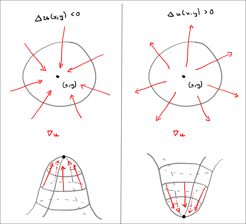
where \(\nabla u(x,y)\) is the gradient vector field, associating to each point in \(\Omega\) the vector of steepest ascent and \(\nabla \cdot\) takes in a vector field and measures for each point how much, for a small region the vectors flow out of it (the divergence). Together, this means that \(\Delta u\) measures the net outflow of the gradient field for each point:

• Positive Laplacian: Means the “uphill” vectors are generally pointing out from the point (like an upside-down cone, a minimum).
• Negative Laplacian: Means the “uphill” vectors are generally pointing in toward the point (like a normal hill, a maximum).

So \(- \Delta u(x,y) = f(x,y) \forall (x,y) \in \Omega\) means the higher \(f(x,y)\) is, the more negative \(-\Delta u(x)\) is, and therefor more points near \((x,y)\) are attracted to it. This is exactly what we would expect from gravitational force! We may see this more clearly, be pushing the signs around: \(\Delta u(x,y) = - f(x,y) \forall (x,y) \in \Omega\)

It might be a good idea to also visualize our mirrored \(f\):

And this might look familiar to an experiment intended to explain gravity, which I assume most have already seen:

example of the laplacian being negative or positive

The influx in the above picture is represented by the laplacian \(\Delta u\). The gray space around the point \((x,y)\) would then be the other values which \(u\) takes on in a neighborhood around \((x,y)\).

---

How can we find \(u\) given the above poisson equation?

We will calculate the solution approximately on a grid

import numpy as np
import plotly.graph_objects as go

N = 10
h = 1 / (N + 1)

square = ([0, 1, 1, 0, 0], [0, 0, 1, 1, 0], [0]*5)

grid_x = [i*h for i in range(1, N+1) for j in range(1, N+1)]
grid_y = [j*h for i in range(1, N+1) for j in range(1, N+1)]
grid_z = [0] * len(grid_x)

boundary = [(x,y,z) 
  for (x,i) in [ (i*h,i) for i in range(N+2) ] 
  for (y,j) in [ (i*h,i) for i in range(N+2) ] 
  for z in [0]
  if i == 0 or j == 0 or i == N+1 or j == N+1
]

fig = go.Figure()

fig.add_trace(go.Scatter3d(x=square[0], y=square[1], z=square[2], mode='lines',
                           line=dict(color='black', width=4), name='Unit Square'))
fig.add_trace(go.Scatter3d(x=grid_x, y=grid_y, z=grid_z, mode='markers',
                           marker=dict(size=5, color='blue'), name=f'Interior (N={N})'))
fig.add_trace(go.Scatter3d(
  x=[v[0] for v in boundary],
  y=[v[1] for v in boundary],
  z=[v[2] for v in boundary],
  mode='markers',
  marker=dict(size=5, color='red'),
  name='Boundary'))

fig.update_layout(
    title=f'Unit Square in (x,y) Plane with Grid Points (N={N}, h={h:.4f})',
    scene=dict(xaxis_title='X', yaxis_title='Y', zaxis_title='Z', aspectmode='cube'),
    showlegend=True, width=800, height=800
)

fig.show()

Finite differences — from scratch

The standard approach for numerically solving the Poisson equation on a uniform grid is the finite difference method. We replace the Laplacian with its five-point stencil:

\[ -\Delta u(x_i, y_j) \approx \frac{4u_{i,j} - u_{i-1,j} - u_{i+1,j} - u_{i,j-1} - u_{i,j+1}}{h^2} = f(x_i, y_j) \]

where \(h = \tfrac{1}{N+1}\) is the grid spacing and \((x_i, y_j) = (ih, jh)\) for \(i,j \in \{1,\ldots,N\}\) are the interior nodes. Stacking all \(N^2\) equations in row-major order gives a linear system \(A\mathbf{u} = \mathbf{b}\).

The following implementation builds that system in a purely functional style (no mutable loops, only map, list comprehensions, and reduce).

import numpy as np
import plotly.graph_objects as go
from functools import reduce

N = 30
h = 1 / (N + 1)

def f(x, y):
    rho1 = 3.0 * np.exp(-60 * ((x - 0.25)**2 + (y - 0.25)**2))
    rho2 = 1.5 * np.exp(-60 * ((x - 0.70)**2 + (y - 0.65)**2))
    return 2 * np.pi * (rho1 + rho2)

xs = list(map(lambda i: (i + 1) * h, range(N)))
ys = list(map(lambda j: (j + 1) * h, range(N)))

def idx(i, j): return i * N + j

def stencil_entries(N, h):
    diag  = [(idx(i,j), idx(i,j),    4/h**2) for i in range(N) for j in range(N)]
    left  = [(idx(i,j), idx(i,j-1), -1/h**2) for i in range(N) for j in range(1, N)]
    right = [(idx(i,j), idx(i,j+1), -1/h**2) for i in range(N) for j in range(0, N-1)]
    up    = [(idx(i,j), idx(i-1,j), -1/h**2) for i in range(1, N) for j in range(N)]
    down  = [(idx(i,j), idx(i+1,j), -1/h**2) for i in range(0, N-1) for j in range(N)]
    return diag + left + right + up + down

def add_entry(A, entry):
    r, c, v = entry
    A[r, c] += v
    return A

A = reduce(add_entry,
           stencil_entries(N, h),
           np.zeros((N * N, N * N)))

b = np.array([f(xs[i], ys[j]) for i in range(N) for j in range(N)])

U = np.linalg.solve(A, b).reshape(N, N)

X, Y = np.meshgrid(xs, ys)
fig = go.Figure(data=[
    go.Surface(x=X, y=Y, z=U.T, colorscale='Viridis',
               contours=dict(z=dict(show=True, usecolormap=True, highlightcolor="limegreen")))
])
fig.update_layout(
    title='Solution u(x,y) of −Δu = f  [from scratch, N=30]',
    scene=dict(xaxis_title='x', yaxis_title='y', zaxis_title='u(x,y)'),
    width=750, height=600,
)
fig.show()

---

Using a library: scipy.sparse

Building a dense \(N^2 \times N^2\) matrix becomes prohibitively expensive for large \(N\). The stiffness matrix \(A\) is actually very sparse — each row has at most five non-zero entries.

A slicker way to construct the 2-D Laplacian is via the Kronecker sum:

\[ A = T \otimes I_N + I_N \otimes T, \qquad T = \frac{1}{h^2}\operatorname{tridiag}(-1,\,2,\,-1) \]

scipy.sparse provides both kron and a direct sparse solver, which makes this the preferred approach in practice.

import numpy as np
import scipy.sparse as sp
import scipy.sparse.linalg as spla
import plotly.graph_objects as go

N = 80
h = 1 / (N + 1)

def f(x, y):
    rho1 = 3.0 * np.exp(-60 * ((x - 0.25)**2 + (y - 0.25)**2))
    rho2 = 1.5 * np.exp(-60 * ((x - 0.70)**2 + (y - 0.65)**2))
    return 2 * np.pi * (rho1 + rho2)

e  = np.ones(N)
T1 = sp.spdiags([-e, 2*e, -e], [-1, 0, 1], N, N, format='csr') / h**2

I  = sp.eye(N, format='csr')
A  = sp.kron(T1, I) + sp.kron(I, T1)

xs = np.array([(i + 1) * h for i in range(N)])
ys = np.array([(j + 1) * h for j in range(N)])
b  = np.array([f(xs[i], ys[j]) for i in range(N) for j in range(N)])

U  = spla.spsolve(A.tocsr(), b).reshape(N, N)

X, Y = np.meshgrid(xs, ys)
fig = go.Figure(data=[
    go.Surface(x=X, y=Y, z=U.T, colorscale='Viridis',
               contours=dict(z=dict(show=True, usecolormap=True, highlightcolor="limegreen")))
])
fig.update_layout(
    title='Solution u(x,y) of −Δu = f  [scipy.sparse, N=80]',
    scene=dict(xaxis_title='x', yaxis_title='y', zaxis_title='u(x,y)'),
    width=750, height=600,
)
fig.show()

Note

Both approaches produce the same solution — the gravitational potential \(u\) induced by two mass concentrations located at \((0.25, 0.25)\) and \((0.70, 0.65)\). The sparse solver handles \(N = 80\) (6 400 unknowns) effortlessly, while the dense solver would require storing a \(6400 \times 6400\) matrix. For even larger systems one would switch to an iterative solver such as conjugate gradients (spla.cg) combined with an AMG or ILU preconditioner.

---

Applied FEM: The Cow

In industry, the finite element method is routinely used to identify stress concentrations and structural failure zones before a part is manufactured.

Classically you’d analyze the stress distribution on a simple geometry like:

cans under load over time

a manufactured part during usage

airflow around a beam

We wish to stay closer to acutal, real life applications though. Everyone knows has done this before: you take a cow and you compress it by applying a load on it (in engineering, this is called a “cowpression”, like “cow” and “compression”).

For this classic example in engineering (analogour to the aerodynamic analysis of a cow), we will solve the Poisson equation on a cow mesh. The solution \(u\) will represent the stress distribution on the cow, and the source term \(f\) will represent the applied load.

import numpy as np
import plotly.graph_objects as go
import trimesh
mesh = trimesh.load_mesh('../../assets/lowpolycow/cow.obj')
mesh.apply_transform(trimesh.transformations.rotation_matrix(np.radians(90), [1, 0, 0]))
mesh.apply_transform(trimesh.transformations.rotation_matrix(np.radians(90), [0, 0, -1]))
# visualize the cow mesh
fig = go.Figure(data=[
    go.Mesh3d(
        x=mesh.vertices[:, 0],
        y=mesh.vertices[:, 1],
        z=mesh.vertices[:, 2],
        i=mesh.faces[:, 0],
        j=mesh.faces[:, 1],
        k=mesh.faces[:, 2],
        color='lightblue',
        opacity=0.5,
        name='Cow Mesh'
    )
])
fig.update_layout(
    title='Low-Poly Cow Mesh',
    scene=dict(xaxis_title='X', yaxis_title='Y', zaxis_title='Z'),
    width=800, height=600,
)
fig.show()

Now that we have our cow ready, lets apply a load on it. We will apply a downward load on the top of the cow, which will be represented by a negative source term \(f\) in the Poisson equation. The solution \(u\) will then represent the stress distribution on the cow, with higher values indicating higher stress.

import numpy as np
import scipy.sparse as sp
import scipy.sparse.linalg as spla
import plotly.graph_objects as go

vertices = mesh.vertices
faces = mesh.faces
V = len(vertices)

# --- Cotangent Laplacian ---
rows, cols, vals = [], [], []
for tri in faces:
    for a, b, c in [(0,1,2),(1,2,0),(2,0,1)]:
        va, vb, vc = vertices[tri[a]], vertices[tri[b]], vertices[tri[c]]
        e1, e2 = vb - va, vc - va
        cos_a = np.dot(e1, e2)
        sin_a = np.linalg.norm(np.cross(e1, e2)) + 1e-12
        cot = cos_a / sin_a
        rb, rc = tri[b], tri[c]
        for r, c_, s in [(rb,rc,1),(rc,rb,1),(rb,rb,-1),(rc,rc,-1)]:
            rows.append(r); cols.append(c_); vals.append(0.5 * cot * s)

L = sp.csr_matrix((vals, (rows, cols)), shape=(V, V))

# --- Load: top vertices are SOURCE (high stress) ---
z = vertices[:, 2]
z_top = np.percentile(z, 90)
z_bot = np.percentile(z, 5)

source = np.where(z >= z_top)[0]
fixed  = np.where(z <= z_bot)[0]
free   = np.setdiff1d(np.arange(V), np.union1d(source, fixed))

# Dirichlet: u=1 at top (load), u=0 at bottom (fixed)
u = np.zeros(V)
u[source] = 1.0
u[fixed]  = 0.0

# Modify system: for free nodes solve L_free * u_free = -L_free_to_bc * u_bc
bc = np.union1d(source, fixed)
L_free = L[free][:, free]
rhs = -(L[free][:, bc] @ u[bc])

u_free, info = spla.cg(L_free, rhs, maxiter=10000, rtol=1e-8)
print(f"CG converged: {info == 0}, range: [{u_free.min():.3f}, {u_free.max():.3f}]")
u[free] = u_free

# --- Plot ---
fig = go.Figure(data=[
    go.Mesh3d(
        x=vertices[:, 0],
        y=vertices[:, 1],
        z=vertices[:, 2],
        i=faces[:, 0],
        j=faces[:, 1],
        k=faces[:, 2],
        intensity=u,
        colorscale='Jet',
        cmin=0, cmax=1,
        colorbar=dict(title='Stress u'),
        name='FEM solution'
    )
])
fig.update_layout(
    title='Poisson FEM – Stress Distribution (top load)',
    scene=dict(xaxis_title='X', yaxis_title='Y', zaxis_title='Z'),
    width=800, height=600,
)
fig.show()

CG converged: True, range: [0.000, 1.000]

And this is where i have left of so far… Maybe some day I will finish this.