1000 * 1.05 * 1.03 * 0.92994.98We wish to understand what \(\exp(x)\) is. We relate compound interest with sailing and along the way find out what \(\pi\) and \(e\) have in common.
Everyone knows the exponential function \(\exp(x)\), and everyone knows the number \(e\). But what are they really?
In this post, we will explore the exponential map in the context of Lie groups and Lie algebras. We will relate it to sailing, playing minecraft and compound interest, and along the way we will uncover the deep connections between these concepts and the fundamental constants of mathematics.
Traditionally, the exponential function is defined as the limit of compound interest. If you invest an amount of money \(m\) at a certain interest rate \(x\) per year, and the interest is compounded \(n\) times per year, then after one year you will have:
\[ A = m \cdot \left(1 + \frac{x}{n}\right)^{n} \]
As \(n\) approaches infinity, this expression converges to:
\[ A = m \cdot e^{x} \]
The significance of this limit is that it tells us how much money we would have, if we were to compound our interest continuously. In the real world, the best banks can do is decrease the compounding period to a day, or even an hour, but mathematically we can imagine compounding infinitely often, which leads us to the exponential function.
\[ \text{exp}(x) = \lim_{n \to \infty} \left(1 + \frac{x}{n}\right)^{n} \]
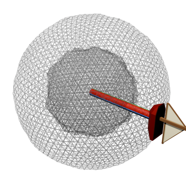
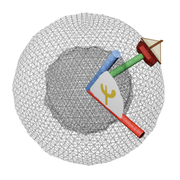
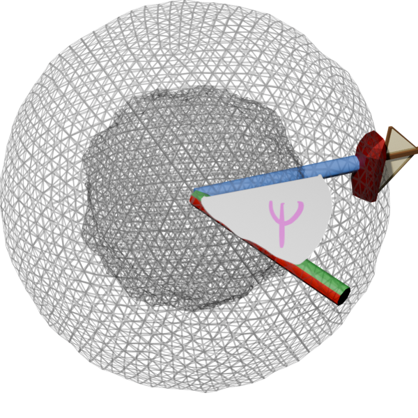
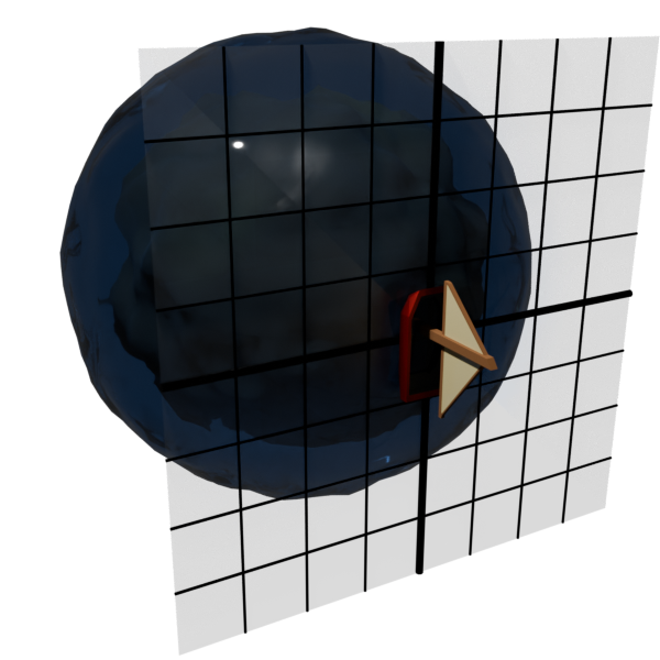
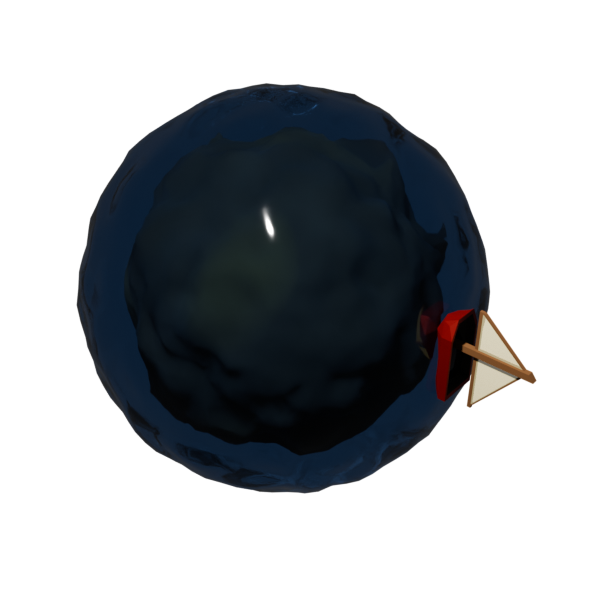
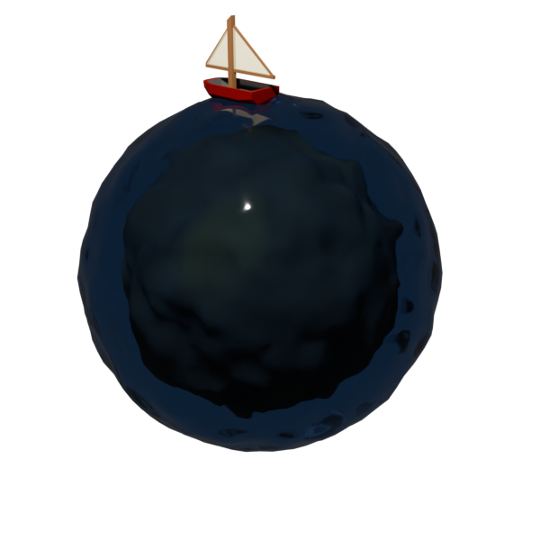
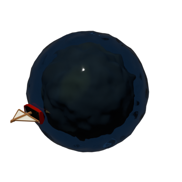
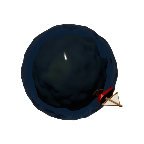
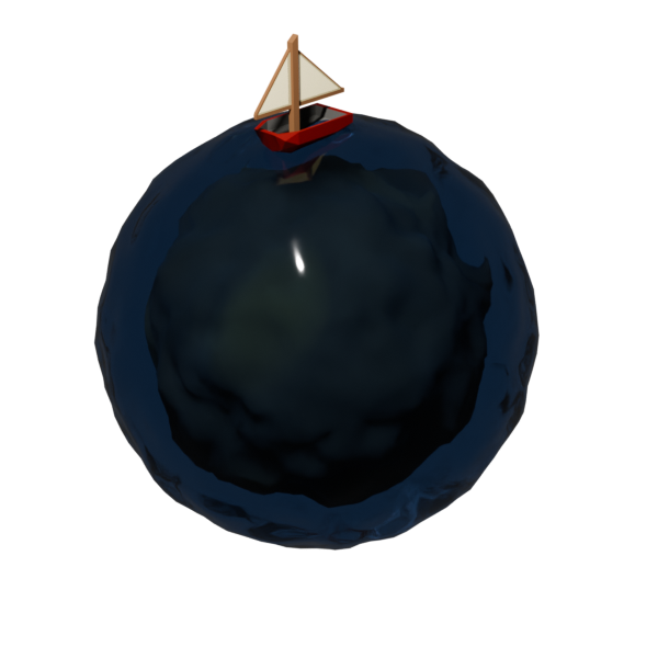
Let us consider a boat sailing on the surface of the Earth, which we can model as a sphere. If we pick some starting point on the globe, we can describe the boat’s position using two angles: latitude \(\textcolor{orange}{\phi}\) and longitude \(\textcolor{purple}{\psi}\) and additionally we can also consider the boat’s orientation, which can be described by a third angle \(\textcolor{teal}{\alpha}\).
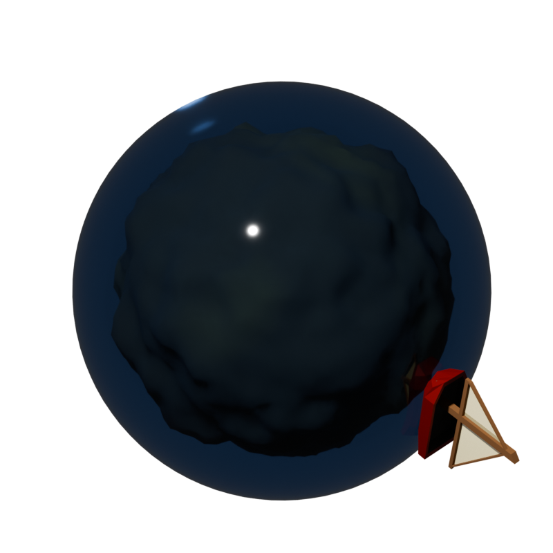
Each possible position of the boat can be represented as a point on the sphere, or equivalently as a pair of angles \((\textcolor{orange}{\phi}, \textcolor{purple}{\psi})\), or as a rotation of the sphere that takes the boat from its starting position to its current position. This rotation/transformation can be represented as a matrix, and the set of all such transformations forms a mathematical structure called a Lie group.
A Lie group is a group that is also a smooth manifold, meaning you can smoothly move between its elements.
Formally: A Lie group \(G\) is a set equipped with
satisfying the usual group axioms (associativity, identity, inverse).
Intuition: You may think of a group as a collection of actions you can do and undo. Walking one step forward and one step backward cancel out; rotating a knob 30° clockwise and then 30° counter-clockwise returns you to where you started. The key is that every action has an undo.
Standard examples:
Weird but useful example: Adding interest to your bank account like the stock market does is a Lie group action: One month you gain say 5%, so if you started with \(x\text{€}\), you will have \(x\text{€} \cdot 1.05\) after that month. The next month you gain 3%, so you will have \(x\text{€} \cdot 1.05 \cdot 1.03\). Now, if the following month, you lose 8%, you will have \(x\text{€} \cdot 1.05 \cdot 1.03 \cdot 0.92\). If you started with \(x=1000\text{€}\), then you would be left with:
1000 * 1.05 * 1.03 * 0.92994.98And you would have lost money. Nontheless, for every gain, there is a loss that undoes it, and for every loss, there is a gain that undoes it, making the process of compounding interest/the stock market a Lie group action on your bank account balance.
As the boat sails, it changes its position on the sphere, and we can represent this change using a Lie group called \(SO(3)\), which describes rotations in three-dimensional space. We have
\[ \begin{aligned} SO(3) &= \{ R \in \mathbb{R}^{3 \times 3} \mid R^T R = I,\ \det(R) = 1 \} \\ &= \{ R_x(\textcolor{teal}{\alpha})\, R_y(\textcolor{orange}{\phi})\, R_z(\textcolor{purple}{\psi}) \mid \textcolor{teal}{\alpha}, \textcolor{orange}{\phi}, \textcolor{purple}{\psi} \in \mathbb{R} \} \end{aligned} \]
The boat’s position at latitude \(\textcolor{orange}{\phi}\) and longitude \(\textcolor{purple}{\psi}\) corresponds to the combined rotation \(R_z(\textcolor{purple}{\psi})\, R_y(\textcolor{orange}{\phi})\), where
\[ \begin{aligned} R_x(\textcolor{teal}{\alpha}) &= \begin{pmatrix} 1 & 0 & 0 \\ 0 & \cos\textcolor{teal}{\alpha} & -\sin\textcolor{teal}{\alpha} \\ 0 & \sin\textcolor{teal}{\alpha} & \cos\textcolor{teal}{\alpha} \end{pmatrix} \\[8pt] R_y(\textcolor{orange}{\phi}) &= \begin{pmatrix} \cos\textcolor{orange}{\phi} & 0 & \sin\textcolor{orange}{\phi} \\ 0 & 1 & 0 \\ -\sin\textcolor{orange}{\phi} & 0 & \cos\textcolor{orange}{\phi} \end{pmatrix} \\[8pt] R_z(\textcolor{purple}{\psi}) &= \begin{pmatrix} \cos\textcolor{purple}{\psi} & -\sin\textcolor{purple}{\psi} & 0 \\ \sin\textcolor{purple}{\psi} & \cos\textcolor{purple}{\psi} & 0 \\ 0 & 0 & 1 \end{pmatrix} \\[8pt] R_z(\textcolor{purple}{\psi})\,R_y(\textcolor{orange}{\phi}) &= \begin{pmatrix} \cos\textcolor{purple}{\psi}\cos\textcolor{orange}{\phi} & -\sin\textcolor{purple}{\psi} & \cos\textcolor{purple}{\psi}\sin\textcolor{orange}{\phi} \\ \sin\textcolor{purple}{\psi}\cos\textcolor{orange}{\phi} & \cos\textcolor{purple}{\psi} & \sin\textcolor{purple}{\psi}\sin\textcolor{orange}{\phi} \\ -\sin\textcolor{orange}{\phi} & 0 & \cos\textcolor{orange}{\phi} \end{pmatrix} \end{aligned} \]
From the starting point of the boat, we can also consider the possible directions in which the boat can sail. Just encoding positions is no fun, we actually would like to sail on our boat after all!
We can sail by varying the angles \(\textcolor{orange}{\phi}\), \(\textcolor{purple}{\psi}\) and \(\textcolor{teal}{\alpha}\), and we can do so by choosing very small changes in these angles, and then applying these more and more times. The smaller the angle, the more we need to apply it, but the better our result will approximate a smooth sailing path on the globe (see the similarity to the limit definition of the exponential function?).
This is similar to video game character movement, where you have a discrete set of controls (e.g. move forward, turn left, turn right) that you can apply repeatedly to navigate the character through the game world. For each frame that passed/tick inside the game which took a time \(\Delta t\) to execute, you apply a small change \(\Delta v\) to the character’s position and orientation, and by applying these changes repeatedly, you can create smooth movement through the game world. If we were to double our tick speed (i.e. halve \(\Delta t\)), we would need to apply these smaller changes \(\Delta v\) twice as often to achieve the “same movement”, albeit with smoother results! This is exactly the same as the limit definition of the exponential function, where we apply smaller and smaller changes more and more often to achieve a smooth transformation.
These directions (\(\color{orange}{\phi}\), \(\color{purple}{\psi}\), \(\color{teal}{\alpha}\) for smaller and smaller angles) form a vector space called the Lie algebra \(\mathfrak{so}(3)\) associated with the Lie group \(SO(3)\). This is also the tangent space of \(SO(3)\) at the identity element, which is the starting point of the boat.
A Lie algebra is a vector space \(\mathfrak{g}\) equipped with a bilinear operation called the Lie bracket \[[\cdot,\cdot] : \mathfrak{g} \times \mathfrak{g} \to \mathfrak{g}\] satisfying:
Intuition: Where a Lie group captures finite, reversible transformations, the Lie algebra captures their infinitesimal, linearised versions — the directions you can move from a given point. If a Lie group is the surface of a globe, the Lie algebra is the tangent plane at the identity, telling you which ways you can sail.
Example — \(\mathfrak{so}(3)\): The Lie algebra of \(SO(3)\) consists of \(3\times 3\) skew-symmetric matrices (i.e. matrices with \(A^T = -A\)), with the bracket given by the matrix commutator \([A,B] = AB - BA\). The three basis elements are the infinitesimal generators of rotations around each axis: \[ L_x = \begin{pmatrix} 0&0&0\\ 0&0&-1\\ 0&1&0 \end{pmatrix},\quad L_y = \begin{pmatrix} 0&0&1\\ 0&0&0\\ -1&0&0 \end{pmatrix},\quad L_z = \begin{pmatrix} 0&-1&0\\ 1&0&0\\ 0&0&0 \end{pmatrix} \] Their brackets reproduce the familiar cross-product relations: \([L_x, L_y] = L_z\), \([L_y, L_z] = L_x\), \([L_z, L_x] = L_y\).
Notice however, that after having moved, say by \(R_y(\frac{\pi}{2})\), applying \(R_x(\frac{\pi}{2})\) no longer corresponds to turning the boat, but rather to being turned by the wind! This is because the transformations do not commute, and the order in which we apply them matters.
The Lie bracket encodes this information, but in the infinitesimal limit.
Recall the videos above: sailing the boat by a tiny angle \(\varepsilon\) over and over again traces out a smooth curve on the globe for \(\color{orange}{\phi}\) and \(\color{purple}{\psi}\) and by also including \(\color{teal}{\alpha}\), the boat can even turn while sailing. The exponential map makes this precise — it turns an infinitesimal direction (an element of the Lie algebra) into a finite transformation (an element of the Lie group), by following that direction for one unit of “time”:
\[ \exp : \mathfrak{g} \longrightarrow G, \qquad \exp(X) = \lim_{n \to \infty} \left(e + \frac{X}{n}\right)^n \]
For matrix Lie groups this limit is just the familiar matrix power series:
\[ \exp(X) = \sum_{k=0}^{\infty} \frac{X^k}{k!} = I + X + \frac{X^2}{2!} + \frac{X^3}{3!} + \cdots \]
Connection to the sailing animation: each generator \(X \in \mathfrak{so}(3)\) describes an infinitesimal rotation — the direction the boat is heading at \(t=0\). Applying it over and over in tiny steps, exactly as in the videos, produces the finite rotation \(\exp(X) \in SO(3)\). This is the same limit we saw for compound interest: more, smaller steps converging to the smooth exponential.
Let \(G\) be a Lie group with Lie algebra \(\mathfrak{g} = T_e G\) (the tangent space at the identity). For each \(X \in \mathfrak{g}\) there is a unique smooth “one-parameter subgroup” \[\gamma_X : \mathbb{R} \to G, \quad \gamma_X(0) = e,\quad \gamma_X'(0) = X\] The exponential map is then defined by \[\exp(X) := \gamma_X(1)\] It satisfies \(\exp(sX) = \gamma_X(s)\) for all \(s \in \mathbb{R}\), and its derivative at \(0\) is the identity: \(d\exp_0 = \mathrm{id}_{\mathfrak{g}}\).
A one-parameter subgroup, although called a “subgroup”, is just a morphism from \((\mathbb{R}, +)\) to \(G\). By requiring \(\gamma_X'(0) = X\), we already uniquely determine \(\gamma_X\) as the solution to the initial value problem, because of the Lie-grouphomomorphism requirement.
The main benefit here is, that we can now choose directions in the Lie algebra given a lie group, and we can (by currying) walk along the geodesic that starts at the identity element of the Lie group and has the chosen direction (and velocity!) for any amount of time we like.
So in minecraft, you are normally given a “spawn point” \(p \in \mathbb{R}^3\). Players can then move around in this world by pressing the W, A, S, D, Space and Shift keys, which correspond to moving forward, left, backward, right, up and down respectively. Assuming that minecraft would be infinitly big and players could move freely without collision detection, this would already form a lie group (in this case \((\mathbb{R}^3, +)\)). But players can also move their camera! So in this case, the underlying manifold would be more like \(\mathbb{R}^3 \times S^2\), where \(S^2\) encodes the camera orientation. By using two angles for \(S^2\), we can define each possible point in this manifold using three numbers \((x,y,z, \phi, \psi)\).
We now still need to twist the \((x,y,z)\)-part of the movement, so that when we press W, we move forward in the direction that our camera is facing, and not just along the \(x\)-axis. We need:
\[ \begin{aligned} (0,0,0, \phi, 0) &\circ (1,0,0, 0, 0) = (\cos(\phi), 0, \sin(\phi), \phi, 0) \\ (0,0,0, \phi, 0) &\circ (0,1,0, 0, 0) = (-\sin(\phi), 0, \cos(\phi), \phi, 0) \\ \dots \\ (0,0,0, 0, \psi) &\circ (1,0,0, 0, 0) = (\cos(\psi), \sin(\psi), 0, 0, \psi) \\ (0,0,0, 0, \psi) &\circ (0,1,0, 0, 0) = (-\sin(\psi), \cos(\psi), 0, 0, \psi) \\ \dots \\ \end{aligned} \]
Here \(\circ\) is the group operation. What if we wish to animate the movement of the player then? We use the exponential map! By currying, we only need to gradually increase \(t\) from \(0\) to \(1\), and we already have a linear interpolation of the movement.
With compound interest, we also also given a Lie group: \((\mathbb{R}_{>0}, \cdot)\). Here \(1\) is the unit (we may also regard it as 100% of our money). “Sailing” here is multiplying by a factor of \(1 + x\), were \(x\) is the interest rate. The Lie algebra is \((\mathbb{R}, +)\), which is again the tangent space of \((\mathbb{R}_{>0}, \cdot)\) at \(1\). We may pick some direction \(X \in \mathbb{R}\), which is the interest rate that we want to apply. If we would set our stepsize/\(\Delta t\) to \(1\), we would only apply the interest once. Kinda like playing a game on 1FPS. If we would set our stepsize to \(0.5\), we would apply the interest twice and so on and in the limit, we want to have a map \(\exp : (\mathbb{R}, +) \times (\mathbb{R}, +) \to (\mathbb{R}_{>0}, \cdot)\) that has \(\frac{d}{dt} \exp(X)(t) = X\) and by abuse of notation, we have \(\exp(X)(1) = \exp(X)\), our trusty old friend from highschool. In particular, we have \(\exp(1) = e\).
As a further consequence, we get that \(\pi = \log(-1)\) for \(\log\) the inverse function (as a morphism of sets) of \(\exp : (\mathbb{R}, +) \to (S^1, \cdot)\), where \(S^1\) is the unit circle in the complex plane. Or another way to see this, is to say that \(2\pi \mathbb{Z} = \text{ker}(exp)\), which means that \(2\pi\) (and \(-2\pi\)) is the answer to the question “how long would I need to travel along the unit circle with unit velocity to get back to where I started, so that any other such length that leads back to the start is just a multiple of this answer?”.
In both cases the problem in the end boils down to calculating the integrals
\[ e = \int_0^1 \gamma_1(t) dt \]
with \(\gamma_1\) the one-parameter subgroup of \((\mathbb{R}_{>0}, \cdot)\) with \(\gamma_1'(0) = 1\), and
\[ 1 = \int_0^{2\pi} \gamma_1(t) dt \]
with \(\gamma_1\) the one-parameter subgroup of \(S^1\) with \(\gamma_1'(0) = 1\).
Moving along a manifold along geodesics is a fundamental operation in geometry and especially in recent times this method has seen a lot of use in machine learning, where the underlying data is often assumed to be a manifold. Especially in the context of optimization, we often want to move along the steepest descent direction, which is a direction in the tangent space of the manifold, like in gradient descent:
Machine learning models are often trained by minimizing a loss function, which measures how well the model is performing on a given task. Take a look at an autoencoder in machine learning:
Basically an autoencoder is just a glorified way to find a “hopefully best” section \(\sigma\) (called decoder) to the retract \(\rho\) (called encoder), as in this figure (here \(\rho\) takes in noisy data and outputs a clean representation, and \(\sigma\) takes in clean data and outputs a compressed representation. Saying they are sections and retracts boils down to \(\sigma \circ \rho = \mathrm{id}\)):
So what we do is, we restrict ourself to a certain subcategory \(\mathcal{C}\) whose objects are the noisy/denoised data manifolds and whose morphisms are some subset of functions between these. We specifically require for all \(f : X \to Y\) in \(\mathcal{C}\) that we have some bolts and nuts that we can turn to tune \(f\) (e.g. the weights), which we reguire to be lie groups (as is common in machine learning, where the weights are often just real numbers, due to using compositions of linear functions and non-linearities weighed by real numbers). We can now define a loss function \(L : X \times X \to \mathbb{R}\), which measures how well a morphism \(f\) is doing at a point by applying \(L(x, f(x))\) or we may form \(\int L(x, f(x)) dx\) to get a more global measure of how well \(f\) performs.
Now, we can use the exponential map to move along the manifold and find those nuts and bolts that minimize the loss function.

