Can the covariance matrix have imaginary eigenvectors?

The covariance matrix

The covariance matrix is commonly defined as:

\[ \begin{aligned} &\text{cov}(X,Y) := \mathbb{E}[(X - \mathbb{E}(X))(Y - \mathbb{E}(Y))^T] \\ &\text{where} \\ &\quad\quad X, Y : (\Omega, \mathcal{F}, P) \xrightarrow{\text{measurable}} (\mathbb{R}^n, \mathcal{B}(\mathbb{R}^n)) \\ &\quad\quad (\Omega, \mathcal{F}, P) \text{ is a probability space} \\ &\quad\quad \mathcal{B}(\mathbb{R}^n) \text{ is the Borel sigma-algebra on } \mathbb{R}^n \end{aligned} \]

If we are given only one random variable \(X\), we can define the covariance matrix of \(X\) as \(\text{cov}(X) := \text{cov}(X,X)\), which is also called the auto-covariance matrix of \(X\). Clearly this auto-covariance matrix is real and symmetric:

\[ \begin{aligned} \text{cov}(X) &= \mathbb{E}[(X - \mathbb{E}(X))(X - \mathbb{E}(X))^T] \\ &= \begin{bmatrix} \mathbb{E}[(X_1 - \mathbb{E}(X_1))^2] & \mathbb{E}[(X_1 - \mathbb{E}(X_1))(X_2 - \mathbb{E}(X_2))] & \cdots & \mathbb{E}[(X_1 - \mathbb{E}(X_1))(X_n - \mathbb{E}(X_n))] \\ \mathbb{E}[(X_2 - \mathbb{E}(X_2))(X_1 - \mathbb{E}(X_1))] & \mathbb{E}[(X_2 - \mathbb{E}(X_2))^2] & \cdots & \mathbb{E}[(X_2 - \mathbb{E}(X_2))(X_n - \mathbb{E}(X_n))] \\ \vdots & \vdots & \ddots & \vdots \\ \mathbb{E}[(X_n - \mathbb{E}(X_n))(X_1 - \mathbb{E}(X_1))] & \mathbb{E}[(X_n - \mathbb{E}(X_n))(X_2 - \mathbb{E}(X_2))] & \cdots & \mathbb{E}[(X_n - \mathbb{E}(X_n))^2] \end{bmatrix} \\ &= \text{cov}(X)^T \end{aligned} \]

As a real symmetric matrix, it cannot have imaginary eigenvalues: Remember that an eigenvalue \(\lambda\) of a matrix \(A\) is defined by the equation:

\[ Av = \lambda v \]

and it therefore can be obtained by solving the characteristic polynomial:

\[ \chi_A(\lambda) = \det(A - \lambda I) = 0. \]

Remember that the determinant of a matrix can be thought of as measuring the “volume” of the parallelepiped spanned by the columns of the matrix. Stating that \(\chi_A\) only has real roots geometrically means that the “volume” of the parallelepiped spanned by the columns of \(A - \lambda I\) can only be zero for real values of \(\lambda\).

Warning

TODO: explain fully why the eigenvalues of a real symmetric matrix are real.

Breaking the symmetry

How would we be able to have a non-symmetric auto-covariance matrix? We would need to have \[ \exists i, j \in \{1, \ldots, n\} : \mathbb{E}[(X_i - \mathbb{E}(X_i))(X_j - \mathbb{E}(X_j))] \neq \mathbb{E}[(X_j - \mathbb{E}(X_j))(X_i - \mathbb{E}(X_i))]. \]

Here, let us first establish without loss of generality that all \(X_i\) are centered, i.e. \(\mathbb{E}(X_i) = 0\) for all \(i\). Then the above condition can be rewritten as:

\[ \exists i, j \in \{1, \ldots, n\} : \mathbb{E}[X_i X_j] \neq \mathbb{E}[X_j X_i]. \]

The multiplication of real random variables is commutative, as it is lifted from the multiplication of real numbers. We will have to consider a non-commutative multiplication to break the symmetry of the auto-covariance matrix, obviously! We can now move over to another ring. In this example, we will consider \(\mathbb{H}\), the ring of quaternions, which is a non-commutative extension of the complex numbers. The quaternions are defined as:

\[ \mathbb{H} := \{a + bi + cj + dk : a, b, c, d \in \mathbb{R}, i^2 = j^2 = k^2 = ijk = -1\} \]

Alternatively, we could mod out the following ideal from the polynomial ring \(\mathbb{R}[i,j,k]\):

\[ \mathbb{H} \cong_\text{Ring} \mathbb{R}[i,j,k] / (i^2 + 1, j^2 + 1, k^2 + 1, ij - k, jk - i, ki - j). \]

We call the elements \(bi + cj + dk\) imaginary, in analogy to the complex numbers. The elements \(a\) are called real.

We can now find a non-symmetric auto-covariance matrix by considering the following random variable, by using \(i j = k\) and \(j i = -k\):

\[ \begin{aligned} &X \in \mathbb{H}^2 \\ &X := \begin{bmatrix} i \\ j \end{bmatrix} \end{aligned} \]

And this gives us the following auto-covariance matrix:

\[ \text{cov}(X) = \begin{bmatrix} 0 & ij \\ ji & 0 \end{bmatrix} = \begin{bmatrix} 0 & k \\ -k & 0 \end{bmatrix} \neq \text{cov}(X)^T. \]

Imaginary eigenvalues

The auto-covariance matrix of \(X = \begin{bmatrix} i \\ j \end{bmatrix}\) has imaginary eigenvalues:

\[ \begin{aligned} \det\left(\begin{bmatrix} -\lambda & k \\ -k & -\lambda \end{bmatrix}\right) &= (-\lambda)(-\lambda) - (k)(-k) \\ &= \lambda^2 - (k)(-k) \\ &= \lambda^2 - (-(k^2)) \\ &= \lambda^2 + k^2 \\ &= \lambda^2 + 1 \end{aligned} \]

So the eigenvalues are the solutions to \(\lambda^2 + 1 = 0\), i.e.

\[ \begin{aligned} &\lambda = i,\ -i \\ \text{or } &\lambda = j,\ -j \\ \text{or } &\lambda = k,\ -k \end{aligned} \]

Rotation of data

To find out the geometric significance of the constructed imaginary eigenvalues, we first need to understand in what way the eigenvalues and eigenvectors of the auto-covariance matrix encode geometric properties of the data.

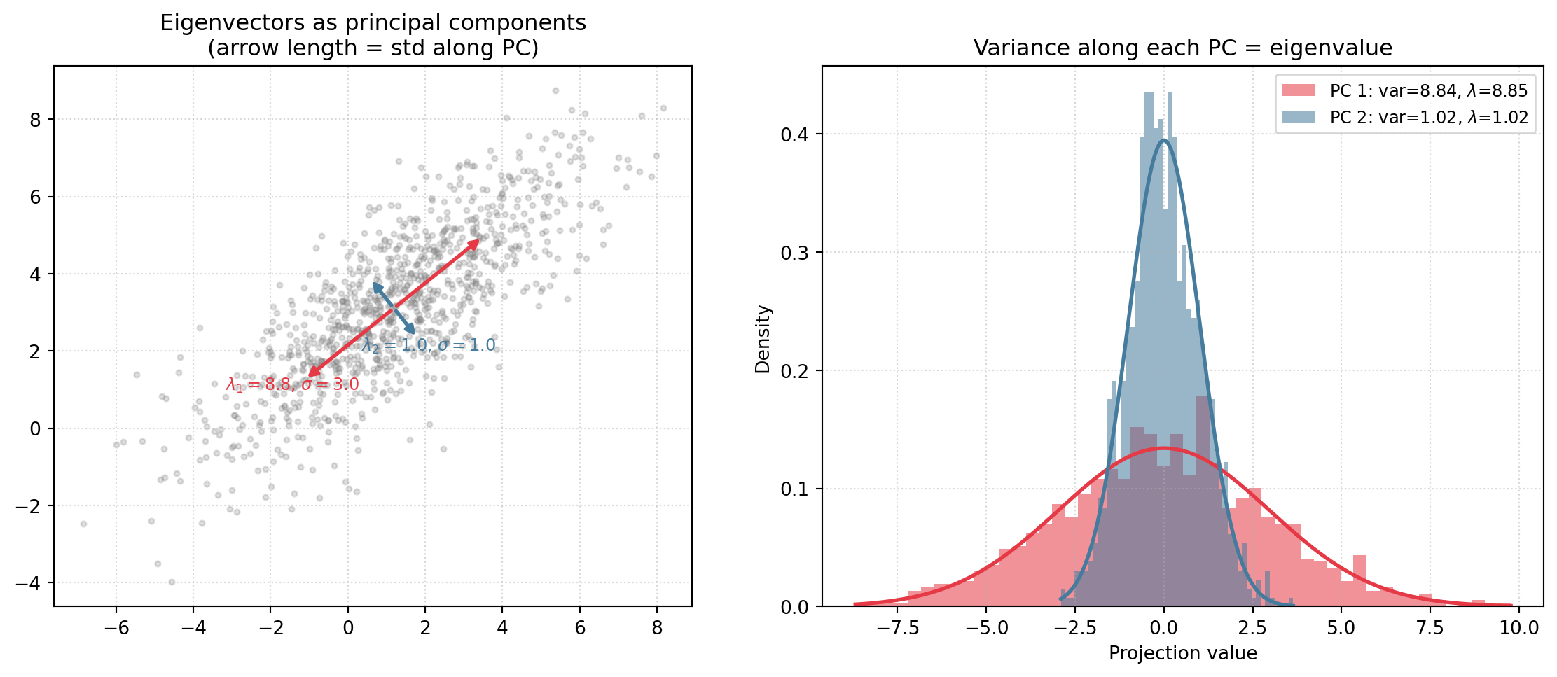
Principal components as eigenvectors

When working with collected samples \(x_1, \ldots, x_N\) of a random variable \(X\), we often work with the sample covariance matrix \(\Sigma_X\), which is defined using the data matrix \(D_X\):

\[ \begin{aligned} &D_X := \begin{bmatrix} x_1^T \\ x_2^T \\ \vdots \\ x_N^T \end{bmatrix} \in \mathbb{R}^{N \times n} \end{aligned} \]

The sample covariance matrix is then defined as:

\[ \begin{aligned} &\Sigma_X := \frac{1}{N} D_X^T D_X \\ &= \frac{1}{N} \sum_{i=1}^N x_i x_i^T \end{aligned} \]

It is well known (see corollary 5.2 https://www.cs.columbia.edu/~djhsu/AML/lectures/notes-pca.pdf), that the eigenvectors of \(\Sigma_X\) are the principal components of the data, and that the eigenvalues of \(\Sigma_X\) are the variances of the data along those principal components. The principal components are obtained by rotating the data in such a way that the variance along each principal component is maximized:

import numpy as np
import matplotlib.pyplot as plt
from scipy.stats import norm

rng = np.random.default_rng(42)

angle = np.radians(40)
R = np.array([[np.cos(angle), -np.sin(angle)], [np.sin(angle), np.cos(angle)]])
X = rng.multivariate_normal([1, 3], R @ np.diag([9, 1]) @ R.T, size=1000)

eigenvalues, eigenvectors = np.linalg.eigh(np.cov(X.T))
eigenvalues, eigenvectors = eigenvalues[::-1], eigenvectors[:, ::-1]
mean = X.mean(axis=0)
colors = ["#e63946", "#457b9d"]

fig, (ax1, ax2) = plt.subplots(1, 2, figsize=(12, 5))

ax1.scatter(X[:, 0], X[:, 1], alpha=0.25, s=8, color="gray")
for i, (lam, vec, c) in enumerate(zip(eigenvalues, eigenvectors.T, colors)):
    std = np.sqrt(lam)
    arrow_kw = dict(arrowstyle="-|>", lw=2, color=c)
    ax1.annotate("", xy=mean + std * vec, xytext=mean, arrowprops=arrow_kw)
    ax1.annotate("", xy=mean - std * vec, xytext=mean, arrowprops=arrow_kw)
    ax1.text(*(mean + (std + 0.4) * vec), rf"$\lambda_{i+1}={lam:.1f}$, $\sigma={std:.1f}$",
             color=c, fontsize=9, ha="center")
ax1.set_aspect("equal")
ax1.grid(True, linestyle=":", alpha=0.5)
ax1.set_title("Eigenvectors as principal components\n(arrow length = std along PC)")

projections = (X - mean) @ eigenvectors
for i, (lam, c) in enumerate(zip(eigenvalues, colors)):
    proj = projections[:, i]
    xs = np.linspace(proj.min(), proj.max(), 300)
    ax2.hist(proj, bins=50, alpha=0.55, color=c, density=True,
             label=rf"PC {i+1}: var={proj.var():.2f}, $\lambda$={lam:.2f}")
    ax2.plot(xs, norm.pdf(xs, scale=np.sqrt(lam)), color=c, lw=2)
ax2.set(xlabel="Projection value", ylabel="Density",
        title="Variance along each PC = eigenvalue")
ax2.legend(fontsize=9)
ax2.grid(True, linestyle=":", alpha=0.5)

plt.tight_layout()
plt.show()

Here, the data matrix would look like this:

\[ D_X = \begin{bmatrix} x_{11} & x_{12} \\ x_{21} & x_{22} \\ \vdots & \vdots \\ x_{N1} & x_{N2} \end{bmatrix} \]

and the sample covariance matrix would be:

\[ \Sigma_X = \frac{1}{N} D_X^T D_X = \frac{1}{N} \begin{bmatrix} x_{11} & x_{21} & \cdots & x_{N1} \\ x_{12} & x_{22} & \cdots & x_{N2} \end{bmatrix} \begin{bmatrix} x_{11} & x_{12} \\ x_{21} & x_{22} \\ \vdots & \vdots \\ x_{N1} & x_{N2} \end{bmatrix} = \frac{1}{N} \begin{bmatrix} \sum_{i=1}^N x_{i1}^2 & \sum_{i=1}^N x_{i1} x_{i2} \\ \sum_{i=1}^N x_{i1} x_{i2} & \sum_{i=1}^N x_{i2}^2 \end{bmatrix} \]

Note

Remember that the standard inner product on \(\mathbb{R}^n\) is defined as \(\langle x, y \rangle = x^T y\), and we have the well known cosine similarity formula: \[ \cos(\theta)\|x\| \|y\| = \langle x, y \rangle = x^T y = \sum_{i=1}^n x_i y_i \] If \(x_{\cdot ,1}\) and \(x_{\cdot, 2}\) in the above example were normed, then the covariance matrix would encode the cosine similarity between the rows of the data matrix, or equivalently the sampled \(x_i\).

The diagonals would clearly just be the lengths (which we assumed to be normed). Dropping our norm assumption, we would therefore be able to obtain the cosine similarity of the data points, by considering the off-diagonal entries of the covariance matrix and dividing them by the square root of the product of the diagonal entries.

Similarly, we can detect the principal components of 3d point clouds. This however crucially only detects the spread of the data along the principal components. If our data has a shape different from a Gaussian blob, PCA will fall short.

import numpy as np
import plotly.graph_objects as go

rng = np.random.default_rng(42)
COLORS = ["#e63946", "#457b9d", "#2a9d8f"]

def add_pca_arrows(fig, X):
    vals, vecs = np.linalg.eigh(np.cov(X.T))
    vals, vecs = vals[::-1], vecs[:, ::-1]
    mean = X.mean(axis=0)
    for i, (lam, vec, c) in enumerate(zip(vals, vecs.T, COLORS)):
        scale = np.sqrt(lam)
        for sign in [1, -1]:
            end = mean + sign * scale * vec
            fig.add_trace(go.Scatter3d(
                x=[mean[0], end[0]], y=[mean[1], end[1]], z=[mean[2], end[2]],
                mode="lines", line=dict(color=c, width=6),
                showlegend=(sign == 1), name=f"PC {i+1} (λ={lam:.2f})"
            ))
            fig.add_trace(go.Cone(
                x=[end[0]], y=[end[1]], z=[end[2]],
                u=[sign * 0.3 * vec[0]], v=[sign * 0.3 * vec[1]], w=[sign * 0.3 * vec[2]],
                colorscale=[[0, c], [1, c]], showscale=False, showlegend=False,
                sizemode="absolute", sizeref=0.4
            ))

layout_kw = dict(margin=dict(l=0, r=0, t=40, b=0), scene=dict(aspectmode="data"))

# Plot 1: 3D Gaussian blob
cov3 = np.array([[4, 2, 0.5], [2, 3, 1], [0.5, 1, 1]])
X1 = rng.multivariate_normal([0, 0, 0], cov3, size=800)

fig1 = go.Figure(layout=layout_kw)
fig1.add_trace(go.Scatter3d(x=X1[:,0], y=X1[:,1], z=X1[:,2], mode="markers",
    marker=dict(size=2, color="#555", opacity=0.5), name="samples"))
add_pca_arrows(fig1, X1)
fig1.update_layout(title="3D Gaussian blob with principal components")
fig1.show()

# Plot 2: xz Gaussian blob with bell-curve bump in y
xz = rng.multivariate_normal([0, 0], [[4, 1], [1, 2]], size=800)
x2, z2 = xz[:, 0], xz[:, 1]
y2 = 2.5 * np.exp(-(x2**2 + z2**2) / 5) + rng.normal(0, 0.1, len(x2))
X2 = np.column_stack([x2, y2, z2])

fig2 = go.Figure(layout=layout_kw)
fig2.add_trace(go.Scatter3d(x=X2[:,0], y=X2[:,1], z=X2[:,2], mode="markers",
    marker=dict(size=2, color="#555", opacity=0.5), name="samples"))
add_pca_arrows(fig2, X2)
fig2.update_layout(title="xz Gaussian blob with bell-curve bump along y: falls short")
fig2.show()

Some standard solutions to this problem are Nonlinear PCA, for example by using kernel methods.

None of these approaches take into account the orientation of our data. It does not matter in which order the data points \(x_i\) are collected and assembled into the data matrix \(D_X\): Assume we permute the data points, resulting in a permuted data matrix \(P D_X\), where \(P\) is a permutation matrix. Then we have \[ \Sigma_{P X} = \frac{1}{N} (P D_X)^T (P D_X) = \frac{1}{N} D_X^T P^T P D_X = \frac{1}{N} D_X^T D_X = \Sigma_X. \]

The geometry of imaginary eigenvalues

We get an obvious injection:

\[ \begin{aligned} \iota &: \mathbb{R}^3 \hookrightarrow \mathbb{H}, \\ \iota(x,y,z) &= xi + yj + zk. \end{aligned} \]

and so we can take the sampled data points \(x_i, \dots, x_N \in \mathbb{R}^3\) from the previous examples and embed them into \(\mathbb{H}^N\). We can now compute the auto-covariance matrix of the result as in the previous chapter and we can compute the eigenvalues of the resulting non-symmetric auto-covariance matrix.

import quaternion

def iota(x, y, z):
    return x * quaternion.x + y * quaternion.y + z * quaternion.z

X1_quat = np.array([iota(*p) for p in X1])
cov_quat = X1_quat[:, np.newaxis] * X1_quat[np.newaxis, :]

Warning

TODO: here I am stuck on how I should best compute the eigenvalues of this matrix of quaternions using NumPy and on what the consequences of the resulting eigenvalues are for the geometry of the data.